The following are notes taken on lecture 9 of the Harvard CS229br seminar on machine learning theory, concerning causality and fairness in machine learning. Thanks to Prof. Boaz Barak and his team for producing this seminar and sharing it freely.

Causality and Fairness

Causality

Resources

Causality by Judea Pearl is considered seminal in the field of causality. However, the following is mostly adapted from Patterns, Predictions, and Actions: A story about machine learning by Moritz Hardt and Benjamin Recht.

Correlation is not Causation, but what is causation? Typically we say “$A$ causes $B$” when $A$ is an intervention and $B$ is an observation that follows ($e$.$g$. “Smoking causes cancer”). In the context of causal analysis, we don’t worry about the feasibility of some causal variable to be controlled by a real-world intervention, and we instead treat all variables as observations and assume that each can be set to a certain value ($e$.$g$. “Obesity causes heart cancer” is a valid statement, without necessarily considering feasible interventions to alter body-weight such as diet or exercise).

Causality Theory is concerned in understanding the conditions under which correlation does imply causation.

Formally, we denote observables: $A, B, C, D, \dots$ and interventions that set outcomes for observables: $\text{do } A \leftarrow a$ etc. (see Judea Pearl’s “do-calculus” and the “do-operator”). Then, correlation and causality are differentiated by:

\[\begin{align} \textcolor{green}{\text{Correlation: }}& \Pr[B = b \mid \textcolor{green}{A = a}] \\ \textcolor{red}{\text{Causation: }}& \Pr[B = b \mid \textcolor{red}{ \text{do }A \leftarrow a}] \end{align}\]

For example, let’s try to predict heart disease in a person (the following is NOT medical advice): Denote whether the person exercises as $X$, whether they’re overweight with $W$ and whether they have heart disease with $H$. Consider two potential causal models:

Scenario 1: Say the probability a person exercises is a binary distribution with probability one half which we write as $X \leftarrow B\left( \frac{1}{2} \right)$. Say then, that both $W$ and $H$ are dependent on $X$ such that a person that exercises is never overweight and never has heart disease, but a person that doesn’t might suffer from either affliction with probability one half. $W$ and $H$ are independent of each other.

\[\begin{matrix} & & \boxed{X \leftarrow B\left( \frac{1}{2} \right)} & &\\ & \swarrow & & \searrow & \\ \boxed{W \leftarrow \begin{cases} 0, &X = 1 \\ B\left( \frac{1}{2} \right), & X=0 \end{cases}} & & & & \boxed{H \leftarrow \begin{cases} 0, &X = 1 \\ B\left( \frac{1}{2} \right), & X=0 \end{cases}} \end{matrix}\]

Scenario 2: Say the person has a chance, perhaps genetically predisposed, to be overweight with probability one quarter. Assume that overweight people don’t exercise, and otherwise the person exercises with probability two thirds. Assume that people that exercise do not get heart disease, and otherwise they do with probability one half.

\[\boxed{W \leftarrow B\left( \frac{1}{4} \right)} \to \boxed{X \leftarrow \begin{cases} 0, &W=1 \\ B\left( \frac{2}{3} \right), &W=0 \end{cases}} \to \boxed{H \leftarrow \begin{cases} 0, &X=1, \\ B\left( \frac{1}{2} \right), &X=0 \end{cases}}\]

Now lets examine the correlations between variables by listing the probability of all outcomes in each scenario based on the conditional probabilities:

$X$	0	0	0	0	1	1	1	1
$W$	0	0	1	1	0	0	1	1
$H$	0	1	0	1	0	1	0	1
$\Pr_{1}$	$\frac{1}{8}$	$\frac{1}{8}$	$\frac{1}{8}$	$\frac{1}{8}$	$\frac{1}{2}$	0	0	0
$\Pr_{2}$	$\frac{1}{8}$	$\frac{1}{8}$	$\frac{1}{8}$	$\frac{1}{8}$	$\frac{1}{2}$	0	0	0

While the causal assumptions in each scenario are different, the outcomes of the models are the same! However, what if instead of examining correlations, we imposed an intervention to causally set observables ourselves? Then, it turns out, we can distinguish between the causal models!

Say we prevent a person from exercising, regardless of whether they intended to exercise in the first place. What do our models predict? Since scenario $\hspace{0pt}1$ assumes that $X$ causes $W$, setting $X$ should affect the outcome of $W$. In contrast, in scenario $\hspace{0pt}2$ the causal relationship goes in the opposite direction, so setting $X$ should not affect the outcome of $W$. An intervention allows us to overwrite the assignment of the variable:

\[\begin{matrix} & & \cancelto{ \boxed{X \leftarrow 0} }{ \boxed{X \leftarrow B\left( \frac{1}{2} \right)} } & &\\ & \swarrow & & \searrow & \\ \boxed{W \leftarrow \begin{cases} 0, &X = 1 \\ B\left( \frac{1}{2} \right), & X=0 \end{cases}} & & & & \boxed{H \leftarrow \begin{cases} 0, &X = 1 \\ B\left( \frac{1}{2} \right), & X=0 \end{cases}} \end{matrix}\] \[\boxed{W \leftarrow B\left( \frac{1}{4} \right)} \to \cancelto{ \boxed{X \leftarrow 0} }{ \boxed{X \leftarrow \begin{cases} 0, &W=1 \\ B\left( \frac{2}{3} \right), &W=0 \end{cases}} } \to \boxed{H \leftarrow \begin{cases} 0, &X=1, \\ B\left( \frac{1}{2} \right), &X=0 \end{cases}}\]

The predictions are different, and importantly, distinguishable:

$X$	0	0	0	0	1	1	1
$W$	0	0	1	1	0	1	1
$H$	0	1	0	1	1	0	1
$\Pr_{1}^{C}$	$\frac{1}{4}$	$\frac{1}{4}$	$\frac{1}{4}$	$\frac{1}{4}$	0	0	0
$\Pr_{2}^{C}$	$\frac{3}{8}$	$\frac{3}{8}$	$\frac{1}{8}$	$\frac{1}{8}$	0	0	0

For instance,

\[\begin{matrix*}[lcc] &\text{Scenario 1} &\text{Scenario 2}\\ \Pr[W = 1 \mid \textcolor{green}{X = 0}] & \frac{1}{2} &\frac{1}{2} \\ \Pr[W = 1 \mid \textcolor{red}{\text{do }X \leftarrow 0}] & \frac{1}{2} &\textcolor{red}{\frac{1}{4}} \\ \end{matrix*}\]

If we were to observe this scenario, we wouldn’t be able to disambiguate these two causal models. But with an intervention, the outcomes will point us towards the true model.

Causality and Science

This is the motive behind scientific experiments: intervene to alter a single variable regardless of its usual causes, to distinguish between hypotheses regarding its causal relationships.

Estimating Causal Probabilities

Often we know, or assume, the shape of the causality graph, as in the direction of causal relationship or lack thereof between all variables, but lack knowledge of the causal probabilities the define these relationships. We want to compute some $\Pr[A = a \mid \text{do } B \leftarrow b]$ from observations of correlations in the system $\Pr[A=a \mid B = b]$.

However, confounding variables must be controlled for. Take the case of the relationship between $W$ and $H$ in scenario $\hspace{0pt}1$. As they’re not causally related, we don’t expect one to affect another, however, we see that they exhibit a correlation when examining naïve conditional probabilities, which is not present under an intervention:

\[\begin{align} &\Pr[H = 1 \mid \textcolor{green}{W = 0}] &= \frac{1}{6}\\ &\Pr[H = 1 \mid \textcolor{red}{\text{do }W \leftarrow 0}] &=\textcolor{red}{\frac{1}{4}} \\ \end{align}\]

This is due to the effect of $X$ on both $H$ and $W$. $X$ is a confounding variable or confounder, and it creates an implied dependence between the two that might be mistaken for a causal relationship. To get the true causal probability we must control for $X$, meaning we must set its value in our computation:

\[\begin{align} \Pr[H=1\mid\textcolor{red}{\text{do }W \leftarrow 0}] = & \Pr[H=1\mid\textcolor{green}{W=0},\textcolor{orange}{X=0}]\Pr[\textcolor{orange}{X=0}] \\ &+ \Pr[H=1\mid\textcolor{green}{W=0},\textcolor{orange}{X=1}]\Pr[\textcolor{orange}{X=1}] \\ =& \cancelto{ \frac{1}{2} }{ \Pr[H=1\mid\textcolor{green}{W=0},\textcolor{orange}{X=0}] }\cancelto{ \frac{1}{2} }{ \Pr[\textcolor{orange}{X=0}] } \\ &+ \cancelto{ 0 }{ \Pr[H=1\mid\textcolor{green}{W=0},\textcolor{orange}{X=1}] }\cancelto{ \frac{1}{2} }{ \Pr[\textcolor{orange}{X=1}] } \\ =& \frac{1}{4} \end{align}\]

This is a special case of the adjustment formula, which concerns any causal graph and computes causal probabilities from conditional probabilities distributed over all outcomes for the confounders¹.

Adjustment Formula

If $Z$ confounds $X$ and $Y$, then:

\[\underbrace{ \Pr[Y=y\mid\textcolor{red}{\text{do }X \leftarrow x}] }_{ \text{Apriori unknown} } = \sum_{z \in Z}\underbrace{ \Pr[Y=y\mid\textcolor{green}{X=x},\textcolor{orange}{Z=z}] }_{ \text{Known from observations given graph} }\Pr[\textcolor{orange}{Z=z}]\]

Failure Cases for Controls

There are several reasons why controlling for too many variables might be detrimental.

Firstly, notice that when we condition on a variable, we can estimate the conditional $\Pr[Y=y \mid X = x, Z = z]$ only from samples that satisfy these three constraints. When conditioning on many variables, the estimations of these conditional probabilities might become unreliable as the sample pool is segmented further and further.

Secondly, we can also control for variables which result in biased estimations. Take for examples two diseases $X$,$Y$, which both occur independently in the population with probability $p \ll 1$, and all sick people are hospitalized, denoted $Z$.

\[\begin{matrix} \boxed{X \leftarrow B(p)} & & & & \boxed{H \leftarrow B(p)}\\ & \searrow & & \swarrow & \\ & & \boxed{Z \leftarrow \begin{cases} 1, & X=1 \cup Y=1 \\ q\ll 1, & X=0 \cap Y=0 \end{cases}} & & \end{matrix}\]

Out of all hospitalized individuals (some proportion $q$ of the population), a proportion of $p$ have disease $X$, a proportion of $p$ have disease $Y$, and the overlap (the proportion of hospitalized individuals that have both $X$ and $Y$ ) is $2p-p^{2} \approx 2p$.

$X$ and $Y$ are not causally connected and not confounded. Their causal and conditional probabilities are equal. The probability that a person with disease $X$ has disease $Y$ is:

\[\Pr[X=1\mid\textcolor{red}{\text{do }Y \leftarrow 1}]= \Pr[X=1\mid\textcolor{green}{Y=1}] = p\]

However, if one were to mistakenly control for hospitalization $Z$, they would reach a different conclusion!

\[\begin{align} \underbrace{ \Pr[X=1\mid\textcolor{red}{\text{do }Y \leftarrow 1}] }_{ \text{Controlling for Z} } = & \Pr[X=1\mid\textcolor{green}{Y=1},\textcolor{orange}{Z=0}]\Pr[\textcolor{orange}{Z=0}] \\ &+ \Pr[X=1\mid\textcolor{green}{Y=1},\textcolor{orange}{Z=1}]\Pr[\textcolor{orange}{Z=1}] \\ = & \cancelto{ 0 }{ \Pr[X=1\mid\textcolor{green}{Y=1},\textcolor{orange}{Z=0}]\Pr[\textcolor{orange}{Z=0}] } \\ &+ \cancelto{ \approx \frac{p^{2}}{2p} = \frac{p}{2} }{ \Pr[X=1\mid\textcolor{green}{Y=1},\textcolor{orange}{Z=1}] }\cancelto{ 2p }{ \Pr[\textcolor{orange}{Z=1}] } \\ \approx p^{2} \end{align}\]

Berkson’s Paradox

The diseases are not correlated, but if we control for the hospitalized population, they become anti-correlated. Should doctors then infect patients with $X$ to prevent the more serious $Y$? This follows the same logical fallacy as bringing a bomb to a plane yourself because the probability of two bombs on a plane is low.

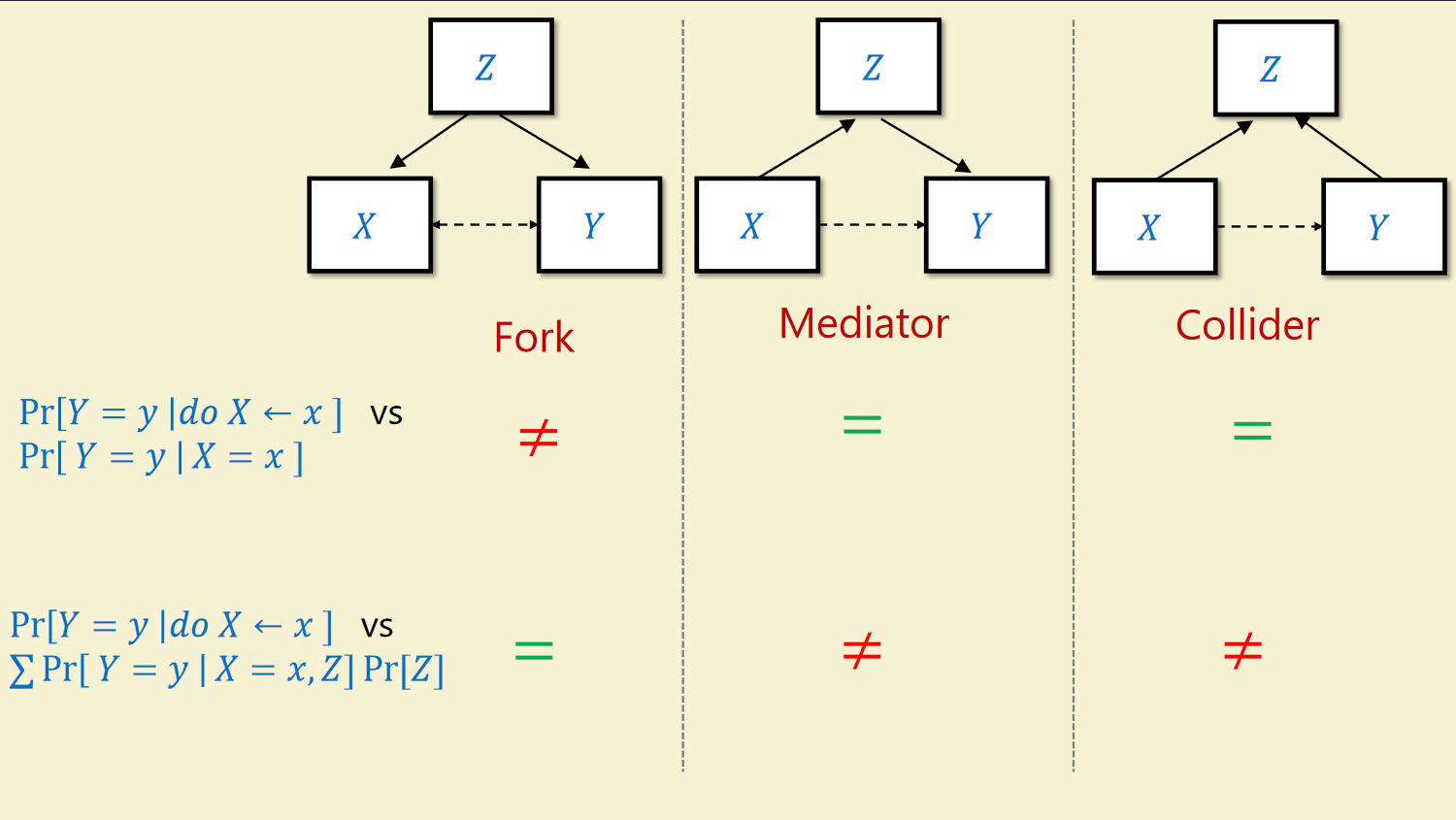
If the causal graph was reversed, and $Z$ became a confounder, it would’ve been crucial to condition on $Z$ to estimate the causal probability. However in this case, it’s crucial that we do not. Hospitalization here is an example of a collider. The effect of variable $Z$ on the causal probability of $X$ and $Y$ can be split into three cases: fork/confounder, mediator and collider. Only in the confounder case should we control for $Z$.

Causal Models

There are two ways to interpret causal models. According to frequentists, the causal probability $\Pr[A\mid \text{do }B]$ is the ratio of experiments where $A$ occurs if we do $B$ and repeat the experiment many times. Bayesians see the causal probability as a counter-factual: We might have already observed the outcome of $A$ without doing $B$, but we can say that $A$ would’ve occurred with probability $\Pr[A\mid \text{do }B]$ in a world where we did do $B$.

When we draw a causal graph for our model, we think of events as lines in a program, following a directed acyclic graph. The graph contains variables as nodes, where the outcomes are determined by functions that can be dependent on other variable nodes or on various instances of exogenous randomness. The graph defines some directed causal relationships but can otherwise be represented as any kind of topological reordering in time.

The Backdoor Criterion

Recall the claim that causal probability and the conditional probability between two variables are only equal when the variables are not confounded. We can define two variables as being confounded if we can find a back door path that connects the dependent variable to an ancestor of the independent variable in either direction.

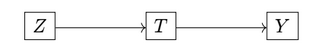
We can see that in this case the causal probability $\Pr[Y=y\mid \text{do }X\leftarrow x]$ is equal to the conditional probability $\Pr[Y=y\mid X=x]$, since we can reorder the directional acyclic graph topologically: If no backdoor path exists, we can topologically sort to “hide” all causes of $X$ from $Y$. Since $X$ is defined as a function of its direct ancestors and some exogenous randomness $U_x$, $X = f(z_{1},\dots, z_{n},u_{x})$, $Y$ is then sampled from a distribution that depends only on $X$ and not on its ancestors: $Y \sim \text{Dist}(x)$. Therefore, the conditional probability is indistinguishable from (equal to) the causal probability.

For example, say we want to design an experiment to test the efficacy of vaccines for COVID$\hspace{0pt}-19$. We might hope that the causal effect of the vaccine intervention on disease contraction $\Pr[C=1\mid \text{do }V \leftarrow 1]$ could be determined from the observed correlation between vaccination and COVID in our cohort $\Pr[C=1\mid V=1]$. However, there exists a backdoor path between contraction and a parent of the vaccination variable: participation in the experiment can be causally related to other contributing causes to contracting COVID.

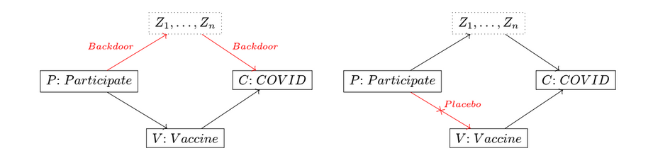
The solution is to control for participation through the introduction of placebo treatment. We randomly assign participants to true treatment and placebo control groups, thereby making vaccination independent of changes in behavior triggered by participation. This way we can observe the average treatment effect by comparing $\Pr[C=1\mid\text{do }V\leftarrow 1,P]$ and $\Pr[C=1\mid\text{do }V \leftarrow 0,P]$ within the participating cohort.

As we saw when we examined fail cases for controls, when we control for (equivalently: condition on) a variable $Z$, we “separate” the graph into a section that feed into $Z$ and the section that follows from $Z$. This cuts off backdoor paths between $Z$’s ancestors and descendants, which allows us to estimate causal effects of the descendant variables it confounded. However, it might result in some spurious relationships when estimating causal effects involving $Z$’s ancestors, which is why we shouldn’t control for colliders and mediators.

Average Treatment Effect and Ignorability

In causal inference we typically consider some binary treatment $T \in { 0,1 }$ and examine the outcomes from the treatment and control groups $Y_{t}:Y\mid \text{do }T \leftarrow t$. We then want to estimate the average treatment effect:

Average Treatment Effect

\[\text{ATE} = \mathbb{E}[Y_{1}]-\mathbb{E}[Y_{0}] = \mathbb{E}[\Pr[Y=1\mid \text{do }T \leftarrow 1]] - \mathbb{E}[\Pr[Y=1\mid \text{do }T \leftarrow 0]]\]

The treatment variable $T$ is dependent on some assignment mechanism dictated by variable $Z$.

When designing experiments, we want the assignment decision to be independent of potential outcomes. This means that we want to know that after conditioning on $Z$, $T$ is independent of the potential causal effect $Y_{t}\mid \text{do }T \leftarrow t$.

RCTs

in our COVID experiment example, it would be ill-advised to assign placebo according to the age of the participants. This is why Randomized Controlled Trials are considered a golden standard in experiment design.

This property is called ignorability, the variables $Y$ and $T$ are called ignorable and $Z$ is called admissible:

\[T \perp (Y_{0},Y_{1})|Z\]

Ignorable variables have the property that the adjustment formula works, that is, the causal effect of $T$ on $Y$ is the expectation over $Z$ of conditional probabilities of $Y$ conditioned on $T$ and $Z$.

\[\Pr[Y=y\mid \textcolor{red}{\text{do }T \leftarrow t}] = \sum_{z \in Z}\Pr[Y=y\mid \textcolor{green}{T=t},\textcolor{orange}{Z=z}]\Pr[\textcolor{orange}{Z=z}]\]

and we can estimate the average treatment effect from observations by conditioning on $Z$:

\[\begin{align} \Pr[Y=1\mid \text{do }T \leftarrow 0] &= \sum_{z \in Z}\Pr[Y=1\mid \cancel{ T=0 }, Z=z]\Pr[Z=z] \\ &= \sum_{z \in Z}\Pr[Y_{0}=1\mid Z=z]\Pr[Z=z] \\ \Pr[Y=1\mid \text{do }T \leftarrow 1] &= \sum_{z \in Z}\Pr[Y=1\mid \cancel{ T=1 }, Z=z]\Pr[Z=z] \\ &= \sum_{z \in Z}\Pr[Y_{1}=1\mid Z=z]\Pr[Z=z] \\ \mathbb{E}[Y_{1}]-\mathbb{E}[Y_{0}] &= \sum_{z \in Z}\Pr[Z=z]\left( \Pr[Y_{1}=1\mid Z=z] - \Pr[Y_{0}=0\mid Z=z] \right) \end{align}\]

Propensity Score

In reality the assignment mechanism $Z$ might not be under our control, but we we can still causal probabilities if we can observe $Z$ and condition on it. We use a measure called the propensity score:

Propensity Score

\[e(z) = \mathbb{E}[T|Z=z] = \Pr[T=1|Z=z]\]

If $Z$ is admissible, we can express the causal probability as a function of $e(z)$.

\[\begin{align} \Pr[Y=y\mid\text{do }T \leftarrow 1] &= \sum_{z \in Z} \Pr[Y=y\mid T=1,Z=z]\Pr[Z=z] \\ &= \sum_{z \in Z} \Pr[Z=z] \frac{\Pr[Y=y,T=1\mid Z=z]}{\Pr[T=1\mid Z=z]} \\ & = \mathbb{E}_{z} \frac{\Pr[Y=y,T=1\mid Z=z]}{e(z)} \\ \mathbb{E}[Y\mid\text{do }T \leftarrow 1] &= \sum_{y} y \Pr[Y=y\mid\text{do }T \leftarrow 1] \\ &= \Pr[Y=1\mid\text{do }T \leftarrow 1] \\ &= \mathbb{E}_{z} \left[ \frac{\Pr[Y=1,T=1\mid Z=z]}{e(z)} \right] \\ &= \mathbb{E}_{z} \left[ \frac{Y\cdot T}{e(z)} \right] \end{align}\]

Propensity Score Matching

In statistical inference, observational experiments often use the propensity score metric to reduce bias due to unknown confounding variables and approximate ignorability. Matching attempts to mimic randomization by pruning the dataset to retain only a sample of treated datapoints which is comparable on all observed covariates to a sample of control datapoints.

Double ML

In reality, as there are many covariates, $Z$ is high-dimensional, and the propensity score is hard to calculate. It’s common to use machine learning models to estimate propensity scores from relatively few samples. Additionally, very small errors in some very small propensity score can translate to very large errors in the estimated causal probabilities due to it’s volatile position in the denominator, an issue that is addressed with the use of “double ML”.

Assume that an outcome $Y$ is composed of some function of $Z$, some treatment effect $\tau$ and some mean-zero noise.

\[Y = \psi(Z) +\tau\cdot T+N\]

Observing $Y$, $T$, $Z$, we can train a model to predict the propensity score $e(z) = \mathbb{E}[T\mid Z=z]$. We can then learn a second model to estimate the outcome dependent on the covariates $f(z)=\mathbb{E}[Y\mid Z=z]$.

\[\begin{align} \mathbb{E}[Y\mid Z=z] &= \mathbb{E}[\psi(Z)\mid Z=z] + \tau \mathbb{E}[T\mid Z=z] + \cancel{ \mathbb{E}[N\mid Z=z] }\\ f(z) &\approx \psi(z)+\tau\cdot e(z) \\ \implies Y-f(z) &\approx \tau \cdot(T-e(z)) \end{align}\]

We can now approximate $\tau$ using linear regression given our observables.

Instrumental Variables

We might run into a problem when some unobserved variables $W$ confound the treatment and outcome. We can still use $Z$ as an instrumental variable to assess the causal effect of $T$ on $Y$, provided that $Z$ does not have any unobserved effect on $Y$ that doesn’t come through $T$.

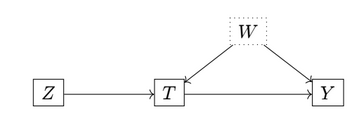
Assuming $Y = \tau\cdot T + f(W)$ and our assumption above, $\text{Cov}(Z,f(W))=0$, we can estimate $\tau$ as:

\[\tau = \frac{\text{Cov}(Z,Y)}{\text{Cov}(Z,T)}\]

Fairness

Resources

The following draws from the book Fairness and Machine Learning by Solon Barocas, Moritz Hardt and Arvind Narayanan, an associated tutorial at NIPS 2017, and the article The (Im)possibility of Fairness by Sorelle A. Friedler, Carlos Scheidegger and Suresh Venkatasubramanian, and focuses on fairness in classification rather than fairness in representation.

Are machine learning models providing utility unevenly across social groups? There have been several high-profile examples of issues with fairness in machine learning.

1) Predicting Risk of Recidivism COMPAS is a company that provides a service to law enforcement in the United States which estimates risk of recidivism for defendants, factoring into decisions to offer bail. An article on the website ProPublica found in $\hspace{0pt}2016$ that the system was racially biased, in the sense that among the defendants who didn’t commit further offenses, African Americans were much more likely to have been labeled higher risk and among those who did reoffend, white people were much more likely to have been labeled lower risk.

2) Gender Detection Buolamwini and Gebru (2018) found that among commercial facial recognition systems that offered gender detection, the true positive rate was $\hspace{0pt}99.7\%$ in white men and only $\hspace{0pt}65.3\%$ in black women, not much better than chance. We will discuss below how discrepancies in classification accuracy can lead to discrimination.

Discrimination exists in society regardless of ML systems, demonstrated in by Bertrand and Mullainathan (2016) who sent out identical CVs to job offers differing only in applicant name, and found they received $\hspace{0pt}50\%$ more callbacks for interviews for white-sounding names, which were more responsive to the quality of the CVs than callbacks for African American names. Further studies show no apparent reduction in discrimination in hiring since.

It seems logical that algorithms can help correct for human bias.

For instance, Gates, Perry and Zorn (2010) argue that more accurate models for predicting defaulters will lower risk for mortgage companies and allow them to lend to more people. However, this also means that if the model is more accurate on some subsections of the population than others, then companies are more likely to lend to people from the former subsections.

Lum and Isaac (2016) examined drug arrests and drug usage in Oakland were police have implemented predictive policing algorithms. They found that the arrests were concentrated in certain neighborhoods while usage was distributed much more uniformly. The demographic distribution of arrested users was similarly concentrated on-nonwhite users in contrast to the uniform demographic distribution of users overall.

Feedback Loops

Lum and Isaac observed a positive feedback loop: The more arrests performed in a neighborhood, the more datapoints pointed to the neighborhood led to more predictions and more arrests.

Defining Unfairness

Definitions of unfairness are constructed around protected classes of properties that are deemed wrong to discriminate against, such as race, age, gender, etc. Any properties that are not proxy to such classes can be used in decision making.

There the measurement of unfairness is performed either in reference to some disparate treatment of groups, or some disparate impact between groups. This creates many valid interpretations of fairness.

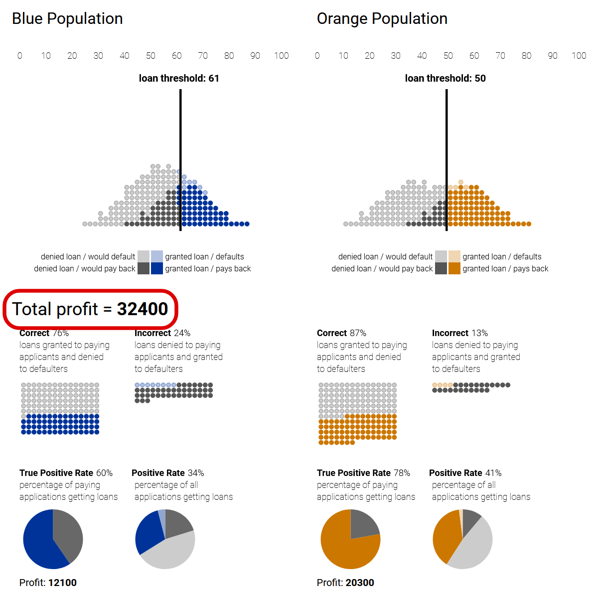
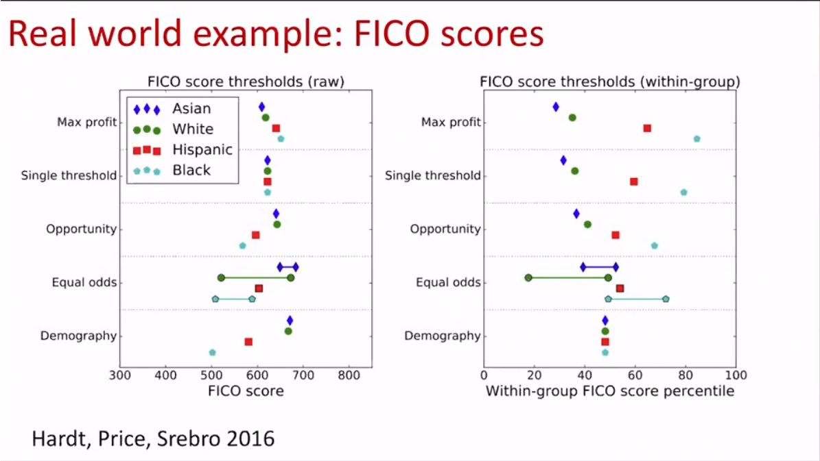
An illustration from Google Research demonstrates in the loan example, how different classification strategies lead to disparate treatment or impact between populations, based on the classifier’s accuracy on each population.

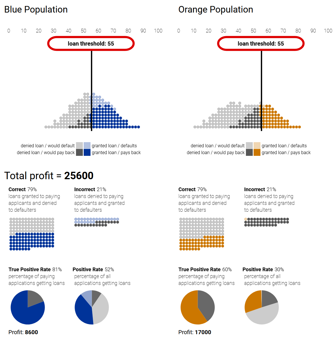
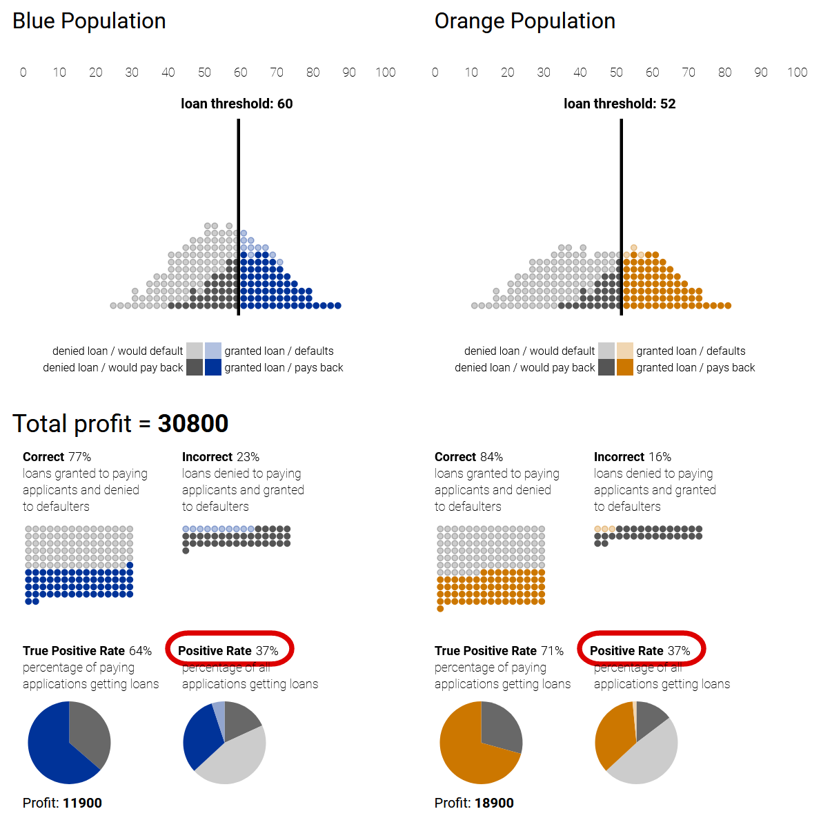
1) Profit-maximizing while disregarding fairness can lead to disparate treatment (loan thresholds) and disparate impact (positive rate) 2) A group-unaware strategy sets the same thresholds for both populations (equal treatment), but still leads to disparate impact. 3) A strategy of demographic parity can ensure equal impact by setting thresholds to equalize the positive rate between the populations, but leads to disparate treatment as the thresholds are set differently. 4) An equal-opportunity strategy ensures quality of impact from the point of view of the applicants (equal true positive rates), but again under disparate treatment.


Profit-Maximizing	Group-Unaware

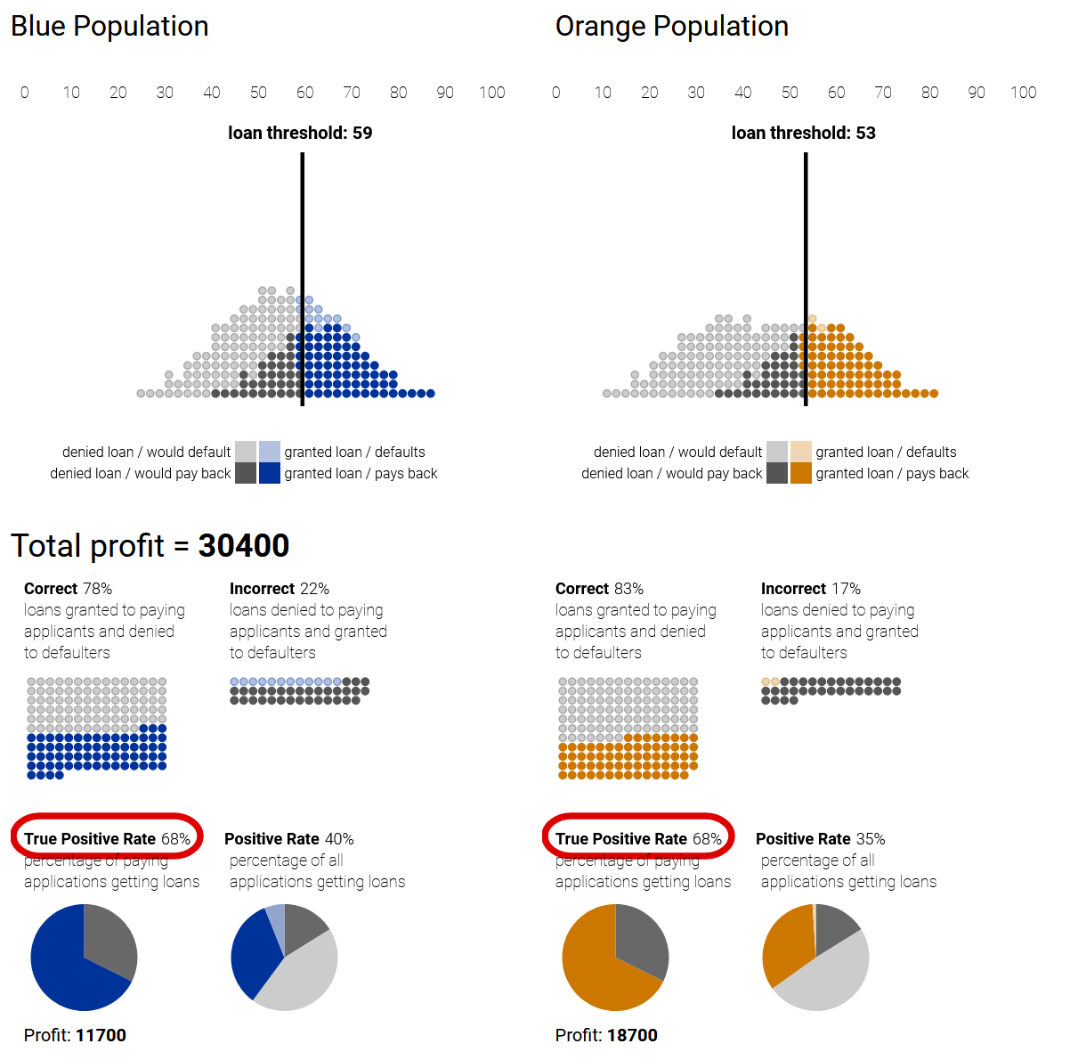Demographic Parity	Equal-Opportunity

Hardt, Price and Srebro (2016) illustrate these tradeoffs in reality looking at FICO credit scores:

Clashing Definitions

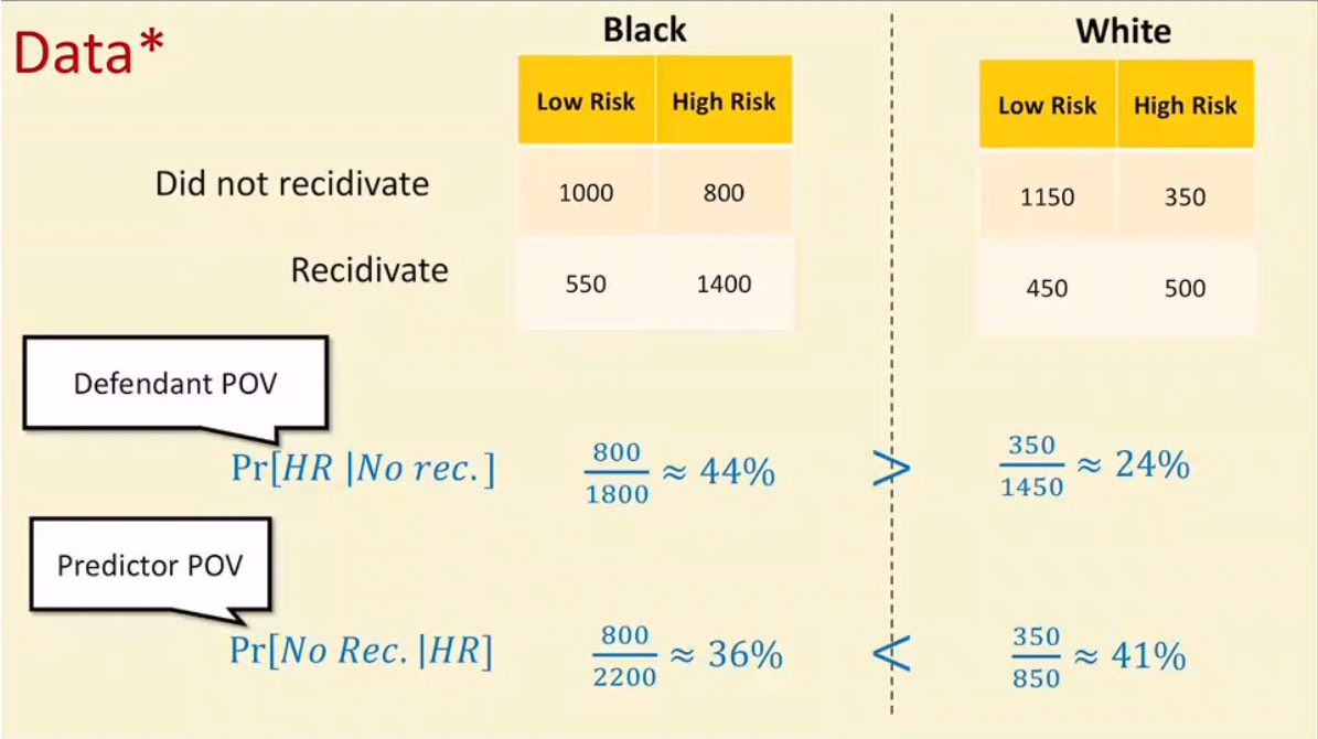
Recall that ProPublica found the COMPAS model led to outcomes where non-recidivists who were white were much less likely to be tagged as high risk. Can COMPAS still be argued to be fair, or biased to favor African Americans?

According to the company’s response, it can. Instead of examining the probability that a high risk defendant didn’t recidivate, they examined the probability that a high-risk defendant did not recidivate. They found that more white high-risk defendants avoided recidivation than African American high-risk defendants!

Different definitions rely on different statistics that often produce clashing results with seemingly equal claim to fairness.

Fairness and Causality

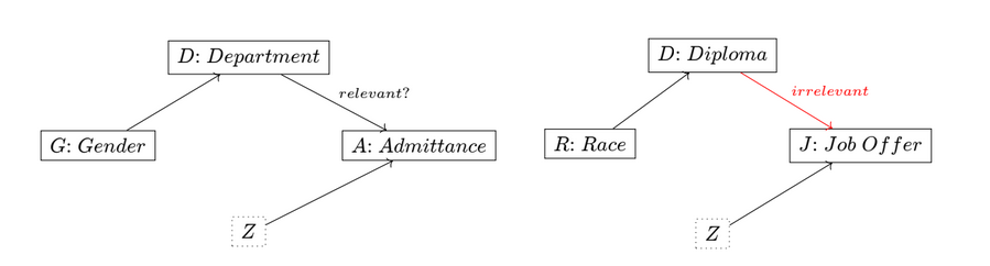
An often cited case, the Berkeley graduate admissions in $\hspace{0pt}1973$ exhibited a similar counter-intuitive results. While $\hspace{0pt}43\%$ of male applicants were admitted as opposed to $\hspace{0pt}35\%$ of female applicants, this rate flipped when examining the admissions within most departments.

Simpson’s Paradox

This is not another case of clashing or confused definitions of fairness. This result stems from lack of ignorability: women were more likely to apply to departments with lower admittance rates.

But is this situation fair? One might argue that the school is not responsible for the applicants’ choice of departments. However, note that the same causal model also corresponds to cases like Griggs v. Duke Power Co. (1971) where a court ruled that since the possession of a high-school diploma was irrelevant to a job offer, the company was discriminating against African Americans by requiring one for the job.

Redlining

This strategy, intentional or not, of producing proxy variables for protected classes to avoid restrictions is nicknamed “redlining” (based on a racist zoning practice in the US).

Fairness in Practice

Since universal observational criteria are not possible for fairness, we rely on our vigilance to check our assumptions regarding:

The representation of data: What was measured and how. Take for example the predictive policing case, where data came from arrests.
The relation to unmeasured inputs and outputs, as we typically care about properties we cannot measure. For instance, hospitals have been shown to perform cost-benefit analysis by proxy of the cost of the medical care going forward. This skewed decision making away from optimizing for health outcomes, especially when controlling for race and gender.
Causal relation of inputs, predictions, and outcomes.

“Value-Free” Algorithms

It’s been often argued that models only reflect biases present in the data, being the biases present in society. However, in reality the model architects make many choices in data collection and model design, which while innocuous at first sight, can introduce more bias or translate bias into discrimination. In addition, as models are deployed in the world, their influence can compound into positive feedback loops.

While sometimes simply collecting more data in the same way will improve results, this is the exception rather than the rule. More often than not, the issue persists unless the pipeline is improved.

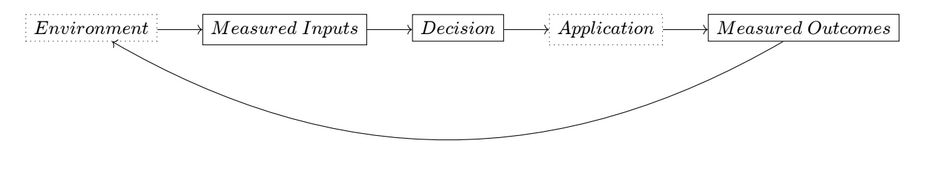
As illustrated by Friedler, Scheidegger and Venkatasubramanian (2021), machine learning deals with four kinds of spaces across two distinctions:

1) Those that contain constructs, such as intelligence or success; and those that contain observations, such as IQ or salary. 2) Those that contain features, such as intelligence or IQ; and those that contain decisions such as success or salary.

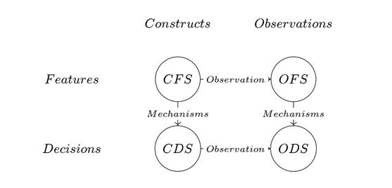
The translations between those spaces, whether through observation or mechanisms of causality, are not trivial nor noiseless, highlighting the importance of decisions made in the process of building predictive models. Even if the model gives the information-theoretically best prediction of the observation-decision output from any observation-feature input, we cannot claim that the model is “value-free”. Value judgements are unavoidable so should be explicit.

For multiple confounders, the set $Z$ that guarantees an unbiased estimation should be chosen carefully. This criterion is called the “Back-Door”, and requires that the elements of $Z$ intercept every path in the graph between the nodes $X$ and $Y$. It might include variables that are not strictly causes of both $X$ and $Y$. See section below. ↩